Computing Complexities – Yassine Moumen

Introduction

Computer is a very powerful tool for solving problems. They are heartless machines that relentlessly obey the laws of logic. A computer cannot think in the way we associate with humans, it is a symbol-manipulating machine that follows a set of stored instructions called a program. It performs these manipulations very quickly and has memory for storing input, lists of commands and output. They do exactly as they are told by following the dictates of logic. Anyone who has worked with computers over the past ten years knows that they are getting faster and better at solving day to day problems. However, it is surprising to learn that there are some easily stated problems that computers cannot satisfactorily solve. In this post, we look at several problems that computers can theoretically solve, but that in practice hard to be solved in an acceptable time. I also explain why some problems seem so hard and why researchers believe that they will never be solved easily.

Can all computational problems be solved by a computer?

There are computational problems that can not be solved by algorithms even with unlimited time. For example, Turing Halting problem. Let us formulate the “To Halt or Not to Halt?” Problem. Given any program and an input for it, determine whether the program with that input will halt or go into an infinite loop. It is a decision problem—that is, it gives a Yes or No answer. Can a computer solve the Halting Problem? The question was described by Alan M. Turing (1912–1954) and in 1936 he gave a definitive negative answer: there is no program that can solve the Halting Problem. There is no way for a computer to determine for any given program, and for any given input into that program, whether the program will halt on that input. If a computer can solve a decision problem, we say the problem is decidable. In contrast, if a computer cannot solve it, we say the problem is undecidable. The Halting Problem is undecidable.

Status of NP Complete problems is another failure story, NP complete problems are problems whose status is unknown. No polynomial time algorithm has yet been discovered for any NP complete problem, nor has anybody yet been able to prove that no polynomial-time algorithm exists for any of them. These problems are not hard because we lack the technology to solve them. Rather, they are hard because of the nature of the problems themselves. They are inherently hard and will probably remain on the outer limits of what we can solve. The interesting part is, if any one of the NP complete problems can be solved in polynomial time, then all of them can be solved. To understand this concept better, let us go back in time to 1736.

A briefer history of mathematics: Euler Cycle

“The Prussian city of Königsberg” was a small town in Russia. The city is on both sides of the Pregel River, a small island at the center of town, and a larger island immediately to its east. Seven bridges connected both islands with each other, as shown in this image:

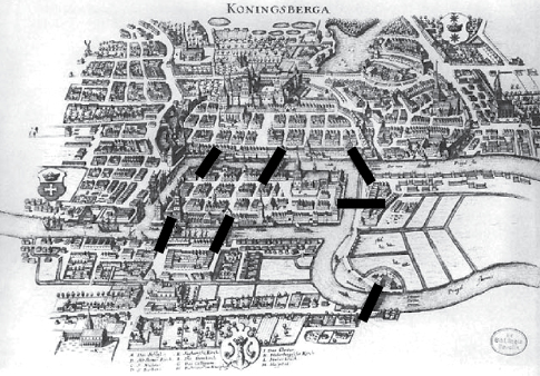
In 1736, the locals were wondering if it was possible to take a tour over the city crossing each bridge exactly once and end up in the same place of start. In attempt to solve it, this riddle was introduced to Leonhard Euler (1707–1783), one of the world’s most important mathematicians of all time. He realized that to find such a path through the seven bridges, we must focus only on what does matter. For example, we do not care if the one, who cross, walk or run, stops for a break, or finish the trip in a week. However, the important information to take in count is the way both islands and the bridges are connected. Euler reformulated the problem in abstract terms, by converting the actual location as a set of nodes connected by links representing the bridges. He then solved the problem analytically rather than by exhaustively listing all possible permutations, and once and for all proved that the Königsberg Bridge Problem was indeed unsolvable.

“My whole method relies on the particularly convenient way in which the crossing of a bridge can be represented. For this I use the capital letters A, B C, D, for each of the land areas separated by the river. If a traveler goes from A to B over bridge a or b, I write this as AB, where the first letter refers to the area the traveler is leaving, and the second refers to the area he arrives at after crossing the bridge. Thus, if the traveler leaves B and crosses into D over bridge f, this crossing is represented by BD, and the two crossings AB and BD combined I shall denote by the three letters ABD, where the middle letter B refers to both the area which is entered in the first crossing and to the one which is left in the second crossing.”
Leonhard Euler

With this method, Euler fundamentally started the field of mathematics known as graph theory. Graph is a mathematical structure used to model pairwise relations between objects, made up of vertices, nodes, or points connected by edges, arcs, or lines. A cycle that passes every edge exactly once is called an Euler cycle. So for any given graph, we may ask if there exists an Euler cycle. This is the Euler Cycle Problem.

What does this have to do with computers and algorithms? Without the information presented in the previous few paragraphs, we might have thought that to determine whether a graph has an Euler cycle we would have to try all possible cycles and see if any cycle crosses every edge exactly once.

For a large graph, there are a tremendous number of cycles to check. Now, with Euler’s trick in hand, we have a new method of determining if there is an Euler cycle. This trick has us simply verifying that every vertex has an even number of edges touching it, which can be done with relatively few operations. Euler’s method has saved us a lot of work. We will always be looking for such tricks.

The problem presented in this section can be solved with algorithms that demand a polynomial number of operations such as n, n², or n × log₂ n operations. Such problems are called polynomial problems. The collection of all polynomial problems is denoted as P. Most polynomial problems can be solved on a modern computer in a feasible or tractable number of operations. Such problems take a feasible amount of time to solve.

In contrast to the feasible problem discussed here, in the next section, we will look at problems that are unsolvable in a reasonable amount of time.

The Traveling Salesman Problem

To get a feel for how hard some problems are, let us introduce the following TSP problem, which is easy to describe. Consider a sales-man who wants to visit five specific cities across Morocco. He wants to visit all the cities in one trip and stop in each city exactly once and then return to the starting point, but he must choose the shortest path in order to save time and money. He looks up the distances between these cities:

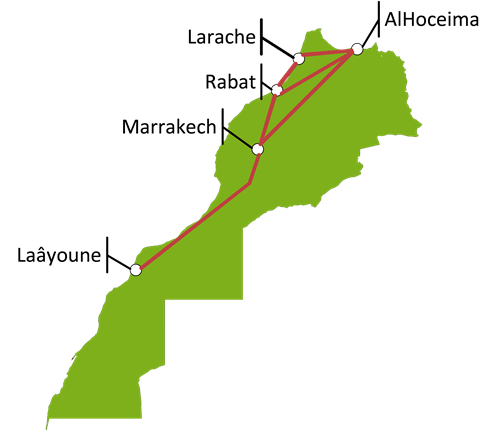
The main question here is which path that connect all cities is the shortest? The obvious and easiest method is to go through all five cities, sum up the distances between the cities (plus the route to the starting point) and see what the total is. Repeat this process until you have all possible routes and then search for the shortest distance of all the possibilities, this method known as Brute-force search.

If we use brute-force search, we must go through all possible routes, but how many there are? First, we have to pick one the five cities to start with; we exclude this one from our list, which left four cities to choose from in the second step. Continuing this way, we conclude that the number of possible routes is: 5 x 4 x 3 x 2 x 1 = 120

For us humans, we consider this a lot of work, but for a computer this operation can take a few microseconds. To generalize this problem, we can imagine the TSP (Traveling Salesman Problem) as a graph with n vertices (points), between two vertices there will be a weighted edge

representing the distance between those two cities ( that is what we call a weighted graph with n vertices). In this graph, we are searching for the shortest path what goes through all cities and return to the starting point. Fallowing the same reasoning as before: there are n possible start cities, n – 1 possible second cities … in the end the number of possible route that we have to check is:

n × (n – 1) × (n – 2) ×•••× 2 × 1

Alternatively, we can write n! (n factorial), which mean that as n gets bigger, n! grows hugely larger.

Let us consider the following case, we have 100 cities for the sales-man to travel to, how many routes are there and how much time needed for a modern computer to search through all of those possible routes?

From our previous conclusion, we have to calculate 100!. We can do this by multiplying 100 times 99 times 98 times 97 . . . times 3 times 2 times 1, that is the human way. Or we can use a computer to do the job for us to obtain the following result:

100! = 93326215443944152681699238856266700490715968264381621468592963895217599993229915608941463976156518286253697920827223758251185210916864000000000000000000000000

It is 9 followed by 157 digits that is the number of potential routes. In order to solve this problem, we would have add up the distances between the 100 cities and compare the result with the other distances already found. Now, imagine that we have a computer that can check one billion routes in one second, the time needed to complete the operation is:

100! / 1000000000 = 93326215443944152681699238856266700490715968264381621468592963895217599993229915608941463976156518286253697920827223758251185210916864000000000000000 seconds.

We divide by 60 = 1555436924065735878028320647604445008178599471073027024476549398253626666553831926815691066269275304770894965347120395970853086848614400000000000000 minutes.

Dividing again by 60 = 25923948734428931300472010793407416802976657851217117074609156637560444442563865446928184437821255079514916089118673266180884780810240000000000000 hours.

Dividing by 24 to get days = 1080164530601205470853000449725309033457360743800713211442048193231685185106827726955341018242552294979788170379944719424203532533760000000000000 days.

to get the years we need to divide by 365 = 2959354878359467043432877944452901461527015736440310168334378611593658041388569114946139776006992588985721014739574573764941185024000000000000 years.

That is 2.9 × 10¹⁴¹ years

Which is bigger than the universe it self in term of age.

2.9 × 10¹⁴¹ years for a computer to figure out the shortest path for 100 cities, which is an unacceptable time. The answer to this problem is possible, but it is impossible to solve this particular riddle in a reasonable amount of time.

This type of problem known as Optimization Problem, “or computational problem in which the object is to find the At the first sight, TSP seems to be limited for a few application areas; however, it can be used to solve tremendous number of problems. Some of the application areas are; printed circuit manufacturing, industrial robotics, time and job scheduling of the machines, logistic or holiday routing, specifying package transfer route in computer networks, and airport flight scheduling.

We have seen that the TSP is essentially unsolvable for any large-sized inputs—that is, it cannot be solved in a reasonable amount of time with our present-day computers. One might try to ignore these limitations by expecting that as computers become faster and faster, NP problems will become easier and easier to solve. Alas, such hopes are futile (AKA, Moore’s Law). As we saw before, the Traveling Salesman Problem for a relatively small input size of n = 100 demands 2.9 × 10142 centuries. Even if our future computers are 10,000 times faster than they are now, our problem will still demand 2.9 × 10138 centuries. This remains an unacceptable amount of time. Conclusion: faster computers will not help us.

How to make a million dollars from this

Once we have one NP-Complete problem, we can easily find others. But how does one find the first NP-Complete problem? In the early 1970s, Stephen Cook of North America and Leonid Levin of Russia independently proved that the Satisfiability Problem is an NP-Complete problem. This theorem, which came to be known as the Cook-Levin Theorem, is one of the most amazing theorems in computer science. The theorem states that all NP problems can be reduced to the Satisfiability Problem. We have seen one of many NP problems. There are currently thousands of known NP problems, some about graphs, some about numbers, some about DNA sequencing, some about scheduling tasks, and so on. These problems come in many different shapes and forms, and yet they are all reducible to the Satisfiability Problem. But wait . . . there’s more! Cook and Levin did not demonstrate that every NP problem now in existence is reducible to the Satisfiability Problem; rather, they showed that all NP problems— even those not yet described—are reducible to the Satisfiability Problem.

At the turn of the millennium, in order to promote mathematics, the Clay Institute declared seven problems in mathematics to be the most important and hardest of their kind. Anyone who solves one of these “Millennium Problems” will receive a million dollars. One of these problems is the P =? NP problem or “is P equal to NP?” We know that P (polynomial) is a subset of NP (nondeterministic polynomial)—that is, every easy problem can be solved in less than a large amount of time. But we can ask the reverse: Is NP a subset of P? Is it possible that every hard NP problem can be solved in a polynomial amount of time? If NP is a subset of P, then P = NP. If NP is not a subset of P, then there is a problem in NP that is not in P and P ≠ NP. The two possibilities are depicted. To win the prize, all you have to do is prove the answer one way or the other.

Introduction

Can all computational problems be solved by a computer?

A briefer history of mathematics: Euler Cycle

The Traveling Salesman Problem

How to make a million dollars from this

Further Reading